Running simulations

You may run a new simulation by adding a new one from scratch, or by cloning an existing simulation.

Prerequisite

If you use credit-based license, make sure that you have enough credit to run the simulation.
To learn more, see credits.

Adding a new simulation

1. From the left panel, click Simulations, then click + ADD SIMULATION on the top right of the page.

2. Fill the fields required in steps #1 to #3 of the wizard, guided by the information described in Simulation parameters.

3. In step #4, select the way you provide the list of base stations involved in your simulation:

   1. Either by reusing the base stations already provisioned on your ThingPark Enterprise account.
      In this mode, the base stations considered in the simulation scope are only the ones associated with an outdoor gateway model. Indoor base stations models (such as Kerlink iFemtocell, Browan femto, Multitech Access Point...) are excluded.

      note

      If you have already filled the "Propagation Environment" and/or "Cable loss" information in ThingPark Enterprise, under your A1 antenna settings, these values are automatically retrieved by the tool besides the BS coordinates.

   2. Or by importing your base stations from a CSV file. To learn more about this option, see Importing base stations by CSV file.

4. In step #5, check-out the base station list on the map.

   caution

   The geographic area covered by the simulation must be less than 10,000 km², otherwise the simulation cannot start. This area is computed according to the minimum and maximum latitude/longitude of the base stations included in the simulation scope.

   The marker colors represent the following cases:

   Marker	Description
   	Some attributes are missing for this base station. You must complete them before launching the simulation
   	The activation of this base station is forced during the execution of the Smart Antenna Selection algorithm (forced activation is enabled). To learn more, see About Smart Antenna Selection.
   	All the attributes are filled for this base station and forced activation is disabled.

   • You may edit the details of a base station by clicking it on the map, then change its attributes then click Save.
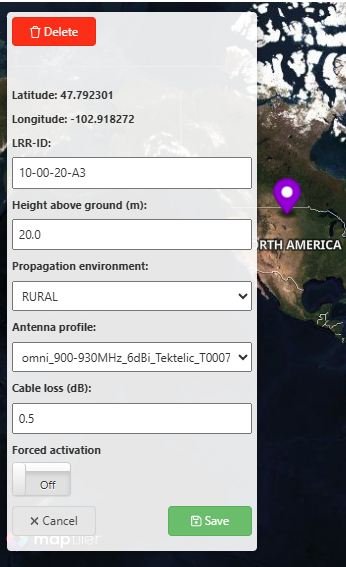
   • To remove a base station from the simulation scope, click it on the map, then click Delete.
   • To add a new base station to the simulation scope, activate the marker tools on the map by clicking on the right. Then, click on the desired location on the map to add a new base station at this location. Some base station attributes are prefilled according to your user preferences, you may change them if needed but you must also fill the missing attributes before launching the simulation.

5. If you want the tool to optimize the list of activated base stations that are required to achieve your coverage targets, activate the Smart Antenna Selection feature. To learn more, see About Smart Antenna Selection.

6. When ready, click START SIMULATION. This button is greyed if some mandatory settings are still missing. You will be notified by email when the simulation results are available. To learn more, see Getting the simulation results.

Simulation parameters

To launch a simulation request, you need to fill in the different input parameters, guided by the table below. All the mandatory inputs are marked by a red asterisk.

Some inputs are already prefilled, either by default settings inherited from the user preferences or inherited from a cloned simulation. You may overwrite any prefilled value if needed.

Parameter	Description
Prediction type	- Safe type of predictions is realistic for all environments, with a slight safety margin < 1dB. - Optimistic type of predictions may be used to simulate the upper bound of the RF coverage using favorable propagation conditions.
Device TX Power	Maximum emission power of the end-device, as supported by its hardware, in dBm. Use a worst-case value if your deployment involves several device models with different transmission capabilities.
Device Antenna Gain	Antenna gain of the end-device, in dBi. Use a worst-case value if your deployment involves several device models with different hardware capabilities.
Default Device Location	Worst-case location of your LoRaWAN end-devices. To learn more, see Device location. Note The simulation results show the expected coverage of all the indoor penetrations deeper than or equal to the selected location. For instance, if the user selects "Indoor daylight", the simulation output will show the predicted coverage of 3 indoor levels: indoor daylight, deep indoor and basement. Note When Smart Antenna Selection is enabled for a device dataset, this default location is used only for devices not associated with any indoor location information in the dataset.
Device Height from ground	Typical setting = 0.5 or 1m to model a device location at the ground floor, which is a kind of worst-case scenario compared to devices located at higher floors. Must be >0 even if a device is located in a basement (in which case set “Device location” = Basement and set “Height from ground” = 0.1: with this setting, the effect of the end-device location is directly modeled in the “basement” indoor penetration losses, not through the antenna height).
Country	Country where your gateways are (or will be) deployed. The country set in the user preferences is used by default but you can change it if needed. The selected country automatically dictates the regulatory limits such as ISM band, Max radiated power and maximum allowed spreading factor.
ISM Band	This parameter defines the LoRaWAN regional profile corresponding to your deployment. By default, it is directly inherited from the country regulations, but you may change it if your country supports several regional profiles (for instance, both EU868 and AS923 are supported in Philippines).
Max Uplink radiated TxPower	Maximum authorized effective isotropic radiated power (EIRP) imposed by the country regulation, for uplink direction, in dBm.
Max Downlink RX1 radiated TxPower	Maximum authorized effective isotropic radiated power (EIRP) imposed by the country regulation, for downlink direction and applicable to RX1 frequencies, in dBm.
Max Downlink RX2 radiated TxPower	Maximum authorized effective isotropic radiated power (EIRP) imposed by the country regulation, for downlink direction and applicable for RX2 frequencies, in dBm.
Uplink Target Packet Error Rate	Maximum acceptable uplink packet error (loss) rate, to be accounted in the link budget analysis of this simulation. Set to 10% by default.
Uplink Noise Rise	Average noise rise over the thermal noise level as seen by the gateway, in dB. - By default, this value is set to 10dB, but it is strongly recommended to set the appropriate value reflecting the noise floor measured by the spectrum analyzer or the gateway onsite. - For more information about spectrum measurements, see the Spectrum Analysis User Guide.
Downlink Noise Rise	Average noise rise over the thermal noise level as seen by the end-device, in dB. This value may be either: - derived from uplink noise rise measurements, taking into account the difference between the end-device location and gateway location. For example, if the end-device is expected to be located deep indoors, it is reasonable to assume 5-10dB lower downlink noise floor than what could be measured by a gateway located outdoors at rooftop. - Alternatively, the expected downlink noise floor could be measured by a spectrum analyzer.
Maximum Uplink Spreading Factor	Maximum authorized UL SF at the cell edge. Note that RF coverage is usually maximized by using the lowest data rate (that is to say, the highest spreading factor) allowed by the corresponding regulatory body (for instance: SF12 in Europe, SF10 in USA). However, some high mobility use cases (tracking, for instance) might require using lower SF for optimal performance under fast fading channel conditions.
Downlink RX2 Spreading Factor	Spreading factor used to send downlink packets over RX2 window. Note that the downlink link budget computed by the tool relies on RX2 window, since it is considered the limiting DL slot from delay standpoint.
Uplink number of transmissions	This parameter defines how many times each uplink frame (that is to say, each FCntUp as per LoRaWAN specification) may be transmitted by a device located at cell edge. For instance, if set to 2, it means that cell edge devices are allowed to send each uplink packet twice.
Digital Elevation Model Type	This field defines the type of digital elevation maps (DEM) used in the simulation: - Either bare-earth digital topography maps for continental Europe, - or JAXA's digital service maps for the rest of the world. The default setting of the DEM type depends on your choice of the Country of operation. If you select a european country having territories outside continental Europe, you should select the right DEM type according to the area covered by your simulation: choose Digital Surface Model if it is outside continental Europe.
Diffraction settings	The default choice depends on the selected DEM: Continental Europe's DTM allows you to simulate the diffraction effect of earth topography for all environments without being negatively impacted by clutter heights (buildings and vegetation). Hence, it is recommended to use the setting "Activated for all environments" only when DEM type = Digital Terrain Mode Europe. For non-european countries, the recommended diffraction setting is "Activated for suburban and rural", as activating the diffraction computation for urban environments may provide pessimistic predictions.
Smart Antenna Selection	By default, this feature is deactivated. Activate it if you want the tool to select the best base stations to cover a defined area or a defined device dataset, among a list of candidate site locations provided in the input csv file. To learn more, see About Smart Antenna Selection.
Polygon	When the Smart Antenna Selection feature is activated, you can draw a polygon on the map to define the target area to be covered. To learn more, see About Smart Antenna Selection.
Device dataset	When the Smart Antenna Selection feature is activated, you can select the device dataset to be covered. To learn more, see About Smart Antenna Selection.
Target coverage percentage	When the Smart Antenna Selection feature is activated, you must set the minimum acceptable coverage ratio of the total area of interest or of the devices of interest. To learn more, see About Smart Antenna Selection.

Importing base stations by CSV file

You may provide the base station list by importing a CSV file.

In step #4 of the simulation creation wizard, click Download sample file to get the CSV template and learn about the format to use.

Click Export BS List if you want some or all of the base stations declared on your ThingPark Enterprise account to constitute the basis of your CSV file. In this case, the exported base stations are only the ones associated with an outdoor gateway model.
Indoor base stations models (such as Kerlink iFemtocell, Browan femto, Multitech Access Point...) will not be exported since the propagation models are only accurate if the base station antenna is located outdoors above the surrounding buildings.

The base station characteristics are uploaded to the simulation through a CSV file. Each line represents one base station. For each base station, you need to fill the following information:

• A unique ID, also known as LRR-ID in ThingPark terminology. You can fill it with the base station ID, its friendly name...
• The base station's GPS coordinates, expressed as latitude and longitude in decimal degree format.
• The base station's height above ground, in meters. Note that this is not the GPS altitude.
• Propagation environment: you must associate each base station with a propagation environment among the values DENSE_URBAN, URBAN, SUBURBAN, and RURAL. To learn more about how to choose the right environment, see Propagation environments.
• Antenna pattern: you can see the list the supported antenna patterns in the Antenna Pattern page of the user interface. The Antenna_pattern column must be filled with the antenna name as written in the Antenna Pattern tab.
• Cable losses in dB. This loss corresponds to the cable, and connector losses. Typical value is around 0.5dB, assuming a short jumper between the gateway connector and the antenna. If longer feeders are installed between the gateway and the antenna, you must compute the right cable losses according to the feeder datasheet (considering the feeder length).
• Forced activation: if the Smart Antenna Selection feature is activated and if this parameter is set to 1, then the base station is selected regardless of its coverage footprint.
  This might be the case of base stations already deployed in the field, which the optimization algorithm should keep activated.

When the CSV file is imported, the tool checks its syntax (comma ',' or semi-column ';' separation and UTF-8 without BOM) and verifies that all the columns are correctly filled with relevant values. If there are errors in the CSV file, they are displayed in the error log (downloadable). When this is the case, you must fix the indicated errors then reload your CSV file.

Cloning a simulation

You can launch a new simulation by cloning an existing one and reusing some of the original settings to avoid re-entering all the configuration settings again.

• The configuration of the cloned simulation is pre-filled with the original simulation data, but you can modify any parameter before launching the new simulation request.
• The base station list is inherited from the original simulation being cloned. Hence, the base stations cannot be reimported, but they can be modified on the map in the last step before launching the simulation, as explained above.
• If the Smart Antenna Selection feature was activated, the area polygon or the dataset used in the original simulation is retrieved by default, but you may redraw another polygon or change the dataset if needed.

---

1. Select the simulation to clone via the checkbox in the first column of the simulation list.
2. Click the button from the top right corner of the page. This button is also present in the detailed page of each simulation.

About Smart Antenna Selection

When the Smart Antenna Selection feature is activated for a given simulation, the Network Coverage tool executes several iterations in the purpose of optimizing/ minimizing the number of base stations needed to reach the targeted coverage requirements.

Coverage requirements may be expressed in two different ways:

• Either a geographic area to be covered, defined by a polygon drawn by the user on the map, when defining a new simulation.

  note

  This polygon is also displayed by the tool in the simulation results. The GPS coordinates of the polygon's corners are also reported in the .json file of the simulation output.

• Or a dataset of LoRaWAN devices to serve. To learn more, see Managing device datasets.

Hence, a typical coverage requirement is to fulfill coverage for at least Z% of the geographic area of interest or at least Z% of the devices defined in the selecyed dataset - Z being defined by the simulation parameter Target coverage percentage.

The optimization algorithm acts as follows:

1. The tool computes the individual coverage provided by each base station and its individual coverage ratio to the geographic area (or devices) of interest.

2. In the first iteration, the tool selects the base stations where forced activation is enabled, if any. These base stations are already pre-selected by the user, for instance because they are already deployed in the field and cannot be decommissioned.

3. Then, from the list of remaining base stations, the tool selects the one having the highest individual coverage ratio (i.e. providing the highest area coverage or device ratio coverage depending on the type of coverage requirements).

4. Then, with this first BS activated, the tool recomputes the incremental coverage of each remaining BS (on top of the coverage provided by the already-activated BS), then activates the one having the highest incremental coverage ratio.

5. Then the process restarts with as many iterations as needed to achieve the target coverage percentage. The simulation stops once the Aggregated coverage ratio >= Target coverage percentage.

   note

   To optimize the simulation time, the calculation also stops when the incremental coverage percentage of each remaining base station is < 0.1% while the aggregated coverage ratio is < Target coverage percentage - 3%.

Optimization results

In the simulation output, the following information is provided:

• In the simulation list:

  • The number of activated BS is displayed out of the total number of candidate base stations. Example means that 22 base stations have been activated by the tool, out of 117 candidate BS.

  • The optimization status is represented by a smiley:

    • A green (happy) face means that the tool has successfully reached the coverage target.
    • An orange face means that the tool could not reach the coverage target with the original candidate BS list. To meet the coverage requirements, additional base station candidates must be provided to a follow-up simulation in order to cover the remaining white spots.
    tip

    Hover your mouse on the smiley displayed in the user interface to see its meaning.

• In the simulation details: List of base stations that have been selected for activation by the tool, among the list of original candidate base stations. This list shows the base stations in the order they have been selected by the tool.

• On the map: Activated base stations are displayed with a marker, whereas base stations that have not be selected (that is to say, deactivated) are marked with a marker. Base stations where forced activation has been enabled are marked with a marker.

Getting the simulation results

Once the simulation is launched, you can follow its status on the Simulations list.

When the simulation is completed, the tool sends a notification email, with a link to the simulation results, as well as the resulting heatmap attached in .kmz format.

If the simulation fails, the credit used at the beginning of the simulation is restored to your account if your license is credit-based.

In the Simulations list, the Optimization column indicates whether the Smart Antenna Selection feature was activated and a smiley specifies if the target coverage percentage was reached, not reached or if no base station can fulfill your coverage requirements.

Exporting simulation data

To export the simulation inputs/outputs, do one of the following:

• From the simulation list, select the simulation you want to export, then click at the top-right corner above the list.
• From the detailed page of your simulation, click the DOWNLOAD button.

The downloaded archive is compressed in .tgz format. You can extract it using a tool like 7zip. The decompressed archive includes the following data:

• A CSV file, entitled <simulation name>.csv, providing the list of all the base stations used as input to this simulation
• A JSON file, entitled <simulation name>.json, providing all the parameter settings used as input to this simulation
• Resulting RF coverage heatmap, available in several formats:
  • Geopackage (.gpkg), compatible with QGIS
  • Google Earth (.kmz)
  • Geotiff (.tiff)
• When Smart Antenna Selection is activated:
  • A CSV file entitled <simulation name>.stats.csv, providing the result of the base station selection process and indicating which base stations were activated by the Smart Antenna Selection mechanism
  • A CSV file entitled <simulation name>.device-dataset-statistics.csv, providing the coverage result of each device included in the input dataset. This file is only relevant when the target coverage requirement consists of a device dataset.